Top Scaling Methods for Market Data Features

Top Scaling Methods for Market Data Features
Scaling financial data is a key step in preparing it for machine learning models, especially in trading applications. Without scaling, features like stock prices and trading volumes, which vary greatly in magnitude, can lead to biased predictions. Proper scaling ensures models focus on meaningful patterns rather than being skewed by large numerical values. Here's a quick breakdown of the most commonly used scaling methods:
- MinMaxScaler: Scales data to a fixed [0, 1] range. It's simple and efficient but sensitive to outliers and struggles with non-stationary data.
- StandardScaler: Centers data around a mean of 0 and standard deviation of 1. Works well for Gaussian-distributed data but is highly affected by outliers.
- RobustScaler: Uses the median and interquartile range, making it resilient to outliers. Ideal for volatile financial datasets.
- PowerTransformer: Adjusts skewed data to resemble a Gaussian distribution. Useful for features with exponential trends or heavy tails.
- MaxDiff Scaling: Normalizes data by dividing by the range (max - min). Fast but amplifies the impact of outliers.
- QuantileTransformer: Maps data to a uniform or normal distribution, reducing the influence of outliers but potentially distorting relationships between variables.
Quick Comparison
| Scaling Method | Handles Outliers | Works with Non-Stationary Data | Best For | Limitations |
|---|---|---|---|---|
| MinMaxScaler | No | No | Features with natural fixed ranges | Sensitive to outliers and future data exceeding range |
| StandardScaler | No | Limited | Gaussian-distributed features | Skewed by outliers, needs periodic updates |
| RobustScaler | Yes | Yes | Volatile or fat-tailed datasets | Slightly higher computational cost |
| PowerTransformer | Partially | Yes | Skewed or heteroscedastic features | Sensitive to extreme outliers |
| MaxDiff Scaling | No | No | Real-time applications | Amplifies outlier influence |
| QuantileTransformer | Yes | Yes | Fat-tailed distributions (e.g., crypto) | Can distort variable relationships |
For trading automation, always fit scalers on training data only to avoid lookahead bias. Tools like Traidies streamline this process by embedding scaling logic directly into workflows, ensuring consistency from backtesting to live trading. Proper scaling can improve model performance significantly - sometimes more than switching to a new algorithm.
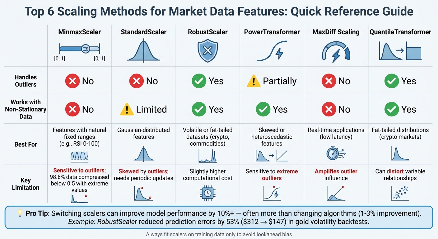
Comparison of 6 Scaling Methods for Financial Market Data
Feature Scaling in Data Science – Normalization vs Standardization
sbb-itb-3b27815
Why Different Scaling Methods Matter
Financial market data is messy and constantly changing. A scaling method that works well for one asset might completely miss the mark for another. Why? It often boils down to three key factors: outliers, non-stationarity, and the underlying distribution.
Let’s start with outliers, which can throw traditional scaling methods completely off track. Markets are full of sudden shocks - think flash crashes, liquidation wicks, or extreme volatility spikes. Techniques like StandardScaler, which rely on the mean and standard deviation, can get skewed by these events. For instance, in a stress test using synthetic data with extreme outliers, 98.6% of the data ended up compressed below the 0.5 mark when MinMaxScaler was applied. Outliers essentially squash normal price movements into a tiny range.
"Extreme outliers make the denominator massive, compressing most of your actual data into a tiny fraction of the available range." - Bala Priya C, Technical Writer
Non-stationarity is another hurdle. Assets don’t stay static - they grow, shrink, and evolve over time. Using global scaling on long-term data can distort historical trends. Take the S&P 500 as an example: it traded around $50 in 1993 but surged to $290 by 2019. A global MinMaxScaler would shrink all 1993 data into a narrow range like [0.00, 0.05], while 2019 data would dominate the upper range [0.90, 1.0]. This creates a problem - moves that were economically significant in 1993 (like a $1 increase, representing a 2% change) might look trivial compared to a $1 move in 2019 (just 0.3%), even though the earlier move carried more weight in context.
Then there’s the issue of fat-tailed distributions. Cryptocurrencies and volatile stocks often experience extreme events far more often than a normal distribution would suggest. In July 2022, Dr. Marios Skevofylakas from Refinitiv analyzed Alphabet Inc. (GOOG.O) data from January 2017 to May 2022. By using an Isolation Forest to weed out outliers before applying scaling, the Root Mean Square Error of a Random Forest model improved from 0.666 to 0.621. This highlights the importance of scaling methods that can preserve normal market behavior without letting rare, extreme events distort the dataset.
The goal of the right scaling method is simple: ensure that a 2% price change in a low-price environment is treated with the same significance as a 2% change in a high-price environment. Linear scaling often falls short here, missing the true economic impact of price shifts under varying conditions. Tackling these challenges head-on is key to choosing the best scaling approach.
1. MinMaxScaler
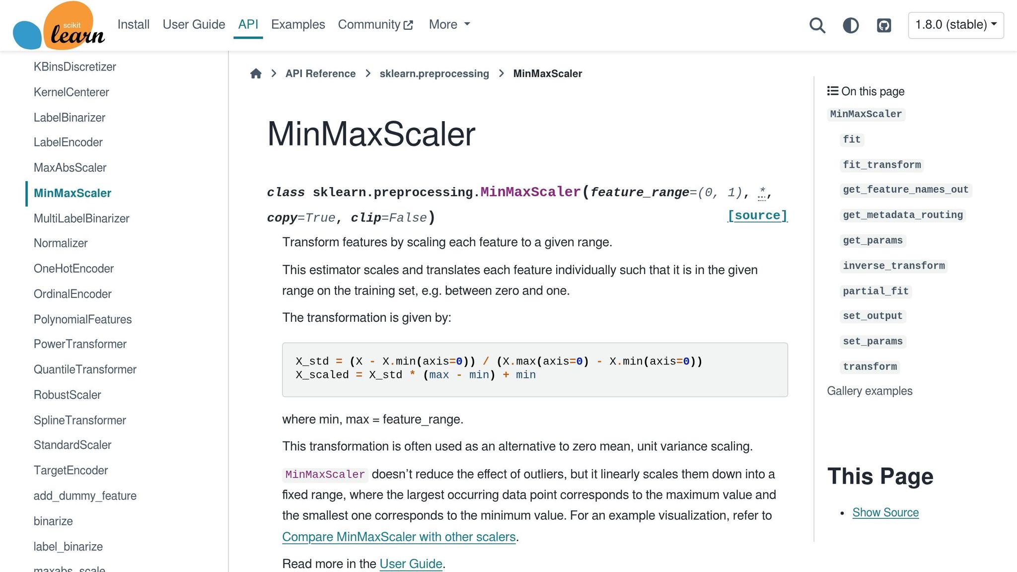
MinMaxScaler is a simple yet widely used technique for scaling data. It works by subtracting the minimum value from each data point and dividing the result by the range (max – min). This process typically scales the data into a fixed range of [0, 1] and keeps the relative distances between data points intact. Its computational efficiency makes it particularly appealing for real-time trading pipelines. However, its simplicity comes with limitations, especially in dealing with outliers and non-stationary data.
Outlier Sensitivity
A major drawback of MinMaxScaler is how easily it can be influenced by outliers. Even a single extreme value can skew the entire scaling process. For instance, in a stress test where most values ranged between 20 and 80, but a few outliers reached 210, the scaler compressed 98.6% of the data into the lower half of the range (below 0.5). This happens because the inflated range denominator forces the majority of the data into a narrower portion of the scale.
Effectiveness for Non-Stationary Data
MinMaxScaler also struggles with non-stationary data, such as financial time series that change over time. Since it relies on fixed scaling boundaries based on historical min/max values, it can create uneven scaling when applied globally. For example, S&P 500 prices ranged from $50 in 1993 to $290 in 2019, causing early data to be compressed into a small range of [0.00, 0.05], while recent data occupied [0.90, 1.0]. This uneven distribution can lead to issues like vanishing gradients in deep learning models, where significant historical fluctuations appear insignificant. Additionally, if future data exceeds the historical maximum or falls below the minimum, the fixed [0, 1] range is no longer valid.
Suitability for Financial Time-Series Features
MinMaxScaler is most effective for features with a defined, natural range, such as technical indicators like the Relative Strength Index (RSI), which typically spans 0–100. It also pairs well with neural networks that use activation functions like sigmoid or tanh, which require inputs within specific intervals. However, it’s not ideal for raw price data or features with fat-tailed distributions, which are common in markets like cryptocurrency. To avoid introducing lookahead bias, always fit the scaler on the training data before applying it to validation or test sets.
2. StandardScaler
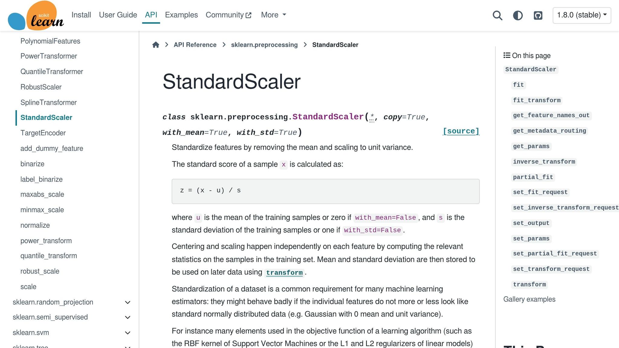
StandardScaler adjusts data by subtracting the mean and dividing by the standard deviation, ensuring a mean of 0 and a standard deviation of 1. This transformation centers data around zero, a format that many machine learning algorithms, including Support Vector Machines, Logistic Regression, and Neural Networks, operate more effectively with. While this method is fundamental in preprocessing, it does come with certain challenges, particularly when dealing with extreme values.
Outlier Sensitivity
One major drawback of StandardScaler is its high sensitivity to outliers. Since both the mean and standard deviation are influenced by extreme values, datasets with outliers can experience distorted scaling. For example, in financial datasets, sudden events like flash crashes or news shocks can inflate the standard deviation. As a result, most "normal" data points may get compressed into a narrow range, such as [-0.2, 0.2], potentially obscuring important patterns. Additionally, when features have outliers on different scales, StandardScaler may not equalize their ranges effectively. One feature might span [-2, 4], while another is confined to [-0.2, 0.2].
"Standardization of a dataset is a common requirement for many machine learning estimators: they might behave badly if the individual features do not more or less look like standard normally distributed data." - scikit-learn documentation
Effectiveness for Non-Stationary Data
StandardScaler works best when the data follows a Gaussian (normal) distribution. However, it struggles with heavily skewed or non-stationary data. Non-stationary data, such as financial time series, often has a mean and variance that shift over time. To handle such scenarios, it's crucial to periodically update the scaling parameters. For dynamic datasets, using rolling normalization - computing Z-scores within a moving window - can be more effective than relying on a global scaler.
Computational Efficiency
From a performance standpoint, StandardScaler is highly efficient. It’s optimized for large-scale data preprocessing, making it a fast choice for scaling tasks. For datasets too large to fit into memory or for continuous data streams, its partial_fit method enables online, batch-by-batch scaling. Additionally, setting copy=False allows in-place computations, reducing memory usage. For sparse datasets, like high-dimensional indicator matrices, it’s important to set with_mean=False to avoid memory issues.
Suitability for Financial Time-Series Features
StandardScaler is particularly effective for features that follow a Gaussian distribution and is well-suited for algorithms that require data to be centered with unit variance. It can also help optimization algorithms, such as Gradient Descent, achieve faster and more reliable convergence by ensuring features are scaled comparably. For instance, in a "Logic Preservation Test" applying a lightweight LSTM model, StandardScaler (Z-Score normalization) outperformed MinMaxScaler for financial time-series convergence. However, if outlier analysis (e.g., boxplots or skewness tests) reveals significant outliers affecting more than 5% of the data, RobustScaler might be a better choice.
Interestingly, among quantitative analysts, there’s an informal rule: while switching from one model (e.g., Random Forest to XGBoost) might improve accuracy by 1–3%, adding well-scaled and engineered features can lead to a 10% improvement in performance.
3. RobustScaler
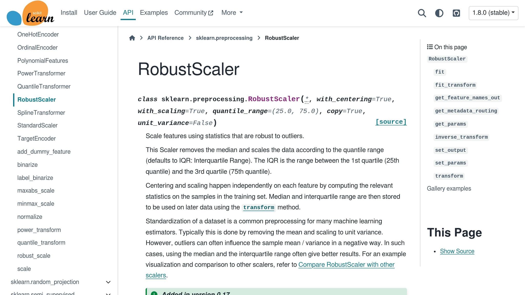
When dealing with outliers, RobustScaler steps in as a more resilient scaling method compared to StandardScaler. Instead of relying on the mean and standard deviation, it uses the median for centering and the interquartile range (IQR) for scaling . By focusing on the middle 50% of the data (the range between the 25th and 75th percentiles), this approach minimizes the impact of extreme values, such as sudden market crashes or price spikes. This makes it a reliable choice for messy, unpredictable financial datasets.
Outlier Sensitivity
One of RobustScaler's standout features is its ability to handle outliers effectively. Unlike MinMaxScaler, which can compress most of the data due to the influence of extreme values, RobustScaler maintains a consistent spread. For example, while outliers only caused minor shifts in the median (0.01) and IQR (0.24), other methods saw a significant inflation in standard deviation (2.01). Importantly, RobustScaler doesn’t clip or collapse outliers like some non-linear transformers do. Instead, it preserves these extreme values, which is critical for models that need to learn from rare but impactful market events.
Effectiveness for Non-Stationary Data
Financial data often exhibits non-stationary behavior, with changing means and variances over time. RobustScaler’s reliance on the central 50% of the data makes it less affected by short-term volatility or structural shifts in the market. This makes it particularly effective for assets with "fat tails", such as Bitcoin and other cryptocurrencies. By ignoring the top and bottom 25% of the data, it captures more stable trends while filtering out noise. To avoid look-ahead bias in time-series applications, always fit the scaler on the training set and apply its parameters to the validation and test sets.
Computational Efficiency
RobustScaler is an affine transformer, meaning it operates efficiently even on large datasets. However, calculating the median and IQR involves sorting, which makes it slightly more computationally demanding than simpler scaling methods. For large-scale sparse datasets, you can optimize performance by disabling centering (with_centering=False) to save memory or using in-place scaling (copy=False) to reduce memory usage. While it may have a slightly higher computational cost, its ability to handle fat-tailed distributions can improve the reliability of optimization algorithms like gradient descent.
Suitability for Financial Time-Series Features
RobustScaler is particularly well-suited for financial time-series data, cryptocurrency markets, and web analytics - domains where extreme anomalies are common . In one regression test using the California housing dataset, its performance was on par with StandardScaler and MinMaxScaler. For trading applications, the default quantile_range of (25, 75) can be adjusted to better align with an asset’s typical behavior. For highly volatile or non-stationary signals, consider using rolling normalization instead of applying global scaling.
4. PowerTransformer (Yeo-Johnson/Box-Cox)

When financial data shows strong skewness or fluctuating variance, the PowerTransformer can reshape the distribution to resemble a Gaussian one. It achieves this using either the Box-Cox or Yeo-Johnson methods, with the transformation parameter (λ) estimated through Maximum Likelihood Estimation. This step is essential for preparing data for models that rely on normally distributed residuals, aligning with the goal of accurate feature scaling.
Outlier Sensitivity
The PowerTransformer adjusts extreme values by reshaping the data distribution, but its λ estimation can be influenced by outliers. As noted in research published by Springer Nature in 2026, "The commonly used Box-Cox and Yeo-Johnson power transformation methods are sensitive to the location, scale, and presence of outliers in the data". A few extreme events, like price spikes or flash crashes, can distort the transformation process. If your dataset includes notable outliers, applying a RobustScaler beforehand can help. Unlike the QuantileTransformer, which entirely neutralizes outliers, the PowerTransformer retains their relative scale while adjusting them into a more Gaussian-like distribution.
Effectiveness for Non-Stationary Data
The PowerTransformer is particularly useful for handling heteroscedasticity. By stabilizing variance and smoothing out exponential trends, it makes data more manageable for models like ARIMA or neural networks. Box-Cox is suitable for strictly positive data, such as asset prices or trading volumes, whereas Yeo-Johnson can handle positive, zero, and negative values, making it a better choice for returns or indicators like MACD.
Computational Efficiency
One potential drawback of the PowerTransformer is the risk of numerical overflow with extreme values or large λs. To avoid issues like data leakage, always include the PowerTransformer within a cross-validation pipeline. Additionally, visually inspecting the transformed data can help confirm its effectiveness. This validation process ties into the implementation steps discussed in later sections.
Suitability for Financial Time-Series Features
The PowerTransformer is well-suited for financial features with heavy tails or exponential growth trends, such as trading volumes during volatile markets or widening price spreads under stress. Both Box-Cox and Yeo-Johnson are monotonic and invertible, enabling the recovery of original data scales after predictions. For smaller datasets (fewer than a few hundred points), the PowerTransformer is less prone to overfitting compared to non-parametric methods like the QuantileTransformer. However, as with other scaling techniques, careful parameter tuning and validation are crucial to adapt to the specific characteristics of financial data. By default, scikit-learn's implementation of PowerTransformer normalizes the output to zero mean and unit variance.
5. MaxDiff Scaling
MaxDiff Scaling takes a straightforward approach by focusing exclusively on the extreme values in a dataset. It normalizes features by dividing each value by the range, which is the difference between the maximum and minimum values. While this method is computationally simple, it can amplify the influence of outliers compared to other techniques like MinMaxScaler or RobustScaler.
Outlier Sensitivity
One of the biggest challenges with MaxDiff Scaling is its high sensitivity to outliers. In financial datasets, for example, a single extreme value - like a sudden market spike - can dominate the scaling process. This often results in most of the data being squeezed into a very narrow range, which can make it less useful for analysis.
Effectiveness for Non-Stationary Data
Since MaxDiff Scaling relies on extreme values, it can fall short when dealing with non-stationary data, such as fluctuating market trends. Applying this method globally may distort the representation of current behaviors. For dynamic conditions, rolling normalization is typically recommended to better adapt to changing data. Choosing the right scaling window becomes critical in these scenarios.
Computational Efficiency
On the plus side, MaxDiff Scaling is incredibly efficient. It only requires basic calculations - finding the maximum, minimum, and their difference - which makes it ideal for fast, real-time applications like algorithmic trading. This simplicity ensures low-latency processing, a key requirement in environments where speed is paramount. However, this computational advantage comes with the trade-off of being more vulnerable to outliers.
6. QuantileTransformer

QuantileTransformer reshapes data to fit a uniform or normal distribution, offering a non-linear alternative to traditional scaling methods. This approach spreads out commonly occurring values while compressing outliers into fixed boundaries. It's especially useful for financial datasets, which often include sharp price swings or sudden volatility changes.
Outlier Sensitivity
This transformer effectively manages outliers by narrowing the gap between extreme and typical values. For instance, during events like flash crashes or sudden market rallies, it maps extreme values to fixed boundaries. This results in value saturation, where significant outliers lose their unique magnitudes and appear indistinguishable. While this helps prevent these extremes from skewing a model's learning process, it comes at the cost of losing detailed information about the size of those extreme shifts.
"This method transforms the features to follow a uniform or a normal distribution. Therefore, for a given feature, this transformation tends to spread out the most frequent values. It also reduces the impact of (marginal) outliers: this is therefore a robust preprocessing scheme." - scikit-learn documentation
Suitability for Financial Time-Series Features
QuantileTransformer is particularly effective for assets with "fat tails", such as cryptocurrencies, where extreme volatility is the norm. It ensures a stable output distribution, making variables measured on different scales comparable. However, this non-linear transformation can distort linear relationships between variables measured on the same scale. For neural networks that expect Gaussian inputs, setting output_distribution='normal' ensures features are mapped correctly.
Computational Efficiency
By default, the transformer uses 1,000 quantiles to discretize the cumulative distribution function and samples 10,000 observations to estimate these quantiles. This non-linear approach does require more computational power than linear scaling methods. For high-frequency trading data, you can tweak the subsample parameter to strike a balance between accuracy and processing speed.
Next, we’ll look at how these scaling techniques can be applied to automated trading systems.
How to Apply Scaling in Trading Automation
When it comes to trading automation, applying scaling methods effectively is key to maintaining both model reliability and performance. For financial time-series data, it's crucial to fit scalers only on the training data and then apply them to the validation and test sets using the transform method. This approach avoids lookahead bias, ensuring that backtest results remain realistic and trustworthy. This disciplined handling of scaling is essential for smooth transitions into automated trading systems.
Focus on stationary features like log returns or differenced data instead of raw prices, which are typically non-stationary. Stationary features allow scalers to learn from stable distributions, avoiding dramatic shifts as market conditions fluctuate.
For practical implementation, scikit-learn Pipelines offer a streamlined solution. These pipelines can chain together scaling, feature selection, and modeling steps, ensuring consistent application of transformations across training, validation, and testing phases. What's even better is that the same pipeline can be deployed in production, so live data undergoes the exact same transformations as the training data.
"Preprocessing shouldn't be treated as an afterthought. The choice of scaler directly affects how features interact within the learning steps, and can make all the difference between a model that generalizes well and one that is biased or unstable".
Tools like Traidies take this a step further by integrating scaling into automated backtesting workflows. For example, when generating MQL5 code for a trading strategy, Traidies embeds proper scaling logic that adapts to historical data while avoiding future data leakage. This modular approach allows users to combine steps like median imputation for missing values, RobustScaler for handling volatile assets, and model training into one automated sequence. This ensures consistency in performance from backtesting to live trading.
One important note: while tree-based models like Random Forest can handle unscaled data, models such as neural networks and distance-based algorithms require scaling. Without scaling, features with larger magnitudes can dominate the learning process in these models. For instance, in gold market volatility backtests, switching from StandardScaler to RobustScaler reduced prediction errors during crisis periods from $312 to $147 - a 53% improvement.
Conclusion
Choosing the right scaling method for financial market data can have a direct impact on the performance of your models. Financial data comes with its own set of challenges - fat-tailed distributions, frequent outliers like flash crashes, and varying scales across features such as stock prices and trading volumes. If not handled correctly, features with larger magnitudes can dominate the learning process, leading to bias. This imbalance can also slow down algorithms that rely on gradient descent, making them less efficient. Addressing these issues is crucial in real-world trading scenarios.
Deciding between StandardScaler, RobustScaler, or QuantileTransformer depends largely on the data's distribution and the specific challenges tied to the asset. For example, in volatile markets like cryptocurrencies or commodities during crisis periods, RobustScaler is often a better choice because it uses the median and interquartile range, making it less sensitive to sudden spikes. On the other hand, StandardScaler can be easily skewed by these outliers, which might make it less reliable in such cases.
Incorporating scaling into automated trading workflows ensures consistency across all stages - from backtesting to live execution. Platforms like Traidies simplify this process by embedding scaling logic directly into generated MQL5 code. They achieve this by fitting scalers exclusively on training data and applying the same transformations consistently across validation, testing, and production environments. This modular approach, which combines scaling with feature engineering and model training, prevents overly optimistic backtests that might fail in live markets. By ensuring uniform application, it not only reduces backtesting bias but also enhances the reliability of models in real trading conditions.
Properly scaled and engineered features can often deliver better results than simply switching to a different algorithm. The choice of scaling method influences training efficiency, sensitivity to anomalies, and overall model dependability. Whether you’re working with neural networks that need bounded inputs or distance-based algorithms sensitive to feature magnitudes, scaling is a critical step for achieving reliable outcomes in automated trading.
FAQs
Which scaler is best for raw prices vs. returns?
For raw prices, the RobustScaler is a great choice because it manages outliers well while keeping the data's scale intact. In contrast, using scalers like StandardScaler can exaggerate the effect of outliers, which can be problematic in unpredictable markets.
When working with returns (such as percentage or log returns), StandardScaler or MinMaxScaler are more suitable. These techniques help by normalizing the data, reducing variance fluctuations, and enhancing model performance by either centering the returns or scaling them within a defined range.
How can I scale time-series data without lookahead bias?
When working with time-series data, maintaining the correct chronological order is critical to avoid lookahead bias. Here's the key: always fit your scaler using only the training data. Once the scaler is trained, use it to transform both the training and test datasets. This approach ensures that the test data is scaled based on parameters derived solely from the training set. To keep things realistic and preserve temporal integrity, split your data chronologically into training and testing sets.
When should I use rolling scaling instead of global scaling?
Rolling scaling is a great approach for handling non-stationary financial data, like stock prices, where statistical properties shift over time. This method normalizes data within a moving window, allowing it to adapt to local trends and reflect evolving market conditions.
In contrast, global scaling relies on statistics from the entire dataset. While useful in some cases, it can distort recent data and hide short-term patterns - making it less effective for markets that are volatile or constantly changing. Rolling scaling ensures that features remain relevant and responsive as conditions evolve.