Risk-Adjusted Portfolio Optimization with MQL5

Risk-adjusted portfolio optimization is about balancing potential returns with risks, aiming to grow capital while minimizing losses. Metrics like the Sharpe Ratio, Sortino Ratio, and CVaR help evaluate performance. Using MQL5, you can automate this process with tools for historical data analysis, risk calculations, and portfolio optimization.

Key takeaways:

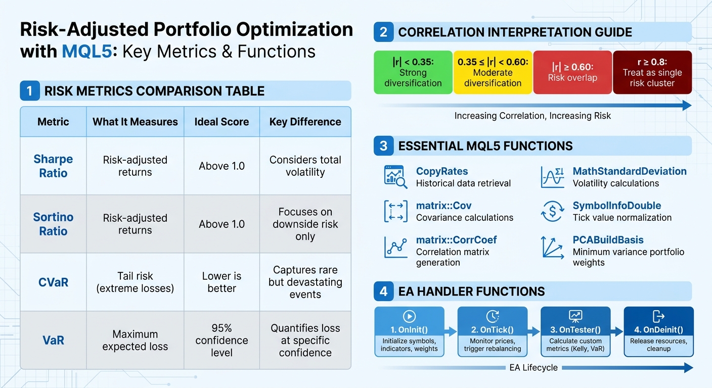
• Sharpe Ratio measures risk-adjusted returns; a score above 1.0 is ideal.
• Sortino Ratio focuses on downside risk.
• MQL5 offers functions like CopyRates for data retrieval and matrix::Cov for covariance calculations.
• The Strategy Tester in MetaTrader 5 visualizes and optimizes strategies using metrics like Sharpe Ratio and Recovery Factor.
• Advanced techniques like Mean-Variance Optimization and Monte Carlo simulations are supported, with Python integration for extended capabilities.

To get started, ensure you have MetaTrader 5, clean historical data, and basic MQL5 programming skills. Automating calculations, normalizing lot sizes based on volatility, and backtesting strategies can help refine your portfolio. Tools like Traidies can simplify code generation and testing, making the process more efficient.

Calculating Risk Metrics in MQL5

Measuring Portfolio Risk with Correlation Matrices

Understanding how assets interact is key to building a well-diversified portfolio. The Pearson correlation coefficient is a tool that measures this relationship, ranging from -1.0 (perfect inverse movement) to +1.0 (perfect synchronization). In MQL5, it's best to use returns data - rather than raw prices - to calculate correlation, as this reduces noise and accounts for non-stationary trends.

MQL5 provides several ways to calculate correlation. The most straightforward method is the built-in matrix::CorrCoef function, which generates a full correlation matrix directly from your data. Alternatively, if you're using the Standard Library, the MathCorrelationPearson function allows you to compute correlations between two arrays. For those who prefer manual calculations, you can implement the Pearson formula by dividing the covariance of two return series by the product of their standard deviations.

Here’s a quick guide to interpreting correlation values:

• |r| < 0.35: Strong diversification
• 0.35 ≤ |r| < 0.60: Moderate diversification
• |r| ≥ 0.60: Risk overlap

For example, if EURUSD and GBPUSD pairs in a multi-EA portfolio show a correlation of r ≥ 0.8, they should be treated as a single risk cluster.

When calculating correlations, logarithmic returns (Log(Price_n / Price_n-1)) are recommended over simple percentage changes. They are more effective for risk estimation methods like Value at Risk (VaR). To streamline the process, automate data export using OnTester() or OnDeinit() events in your Expert Advisor. Save daily profit-and-loss or return data to CSV files for later analysis. You can also create a visual heatmap using OBJ_RECTANGLE_LABEL objects, with green and red colors indicating positive and negative correlations, respectively.

Once you’ve analyzed correlations, use these insights to calculate overall portfolio variance and projected returns.

Computing Portfolio Variance and Expected Returns

After assessing correlations, the next step is calculating portfolio risk and returns. Start by retrieving historical price data using the CopyRates function for your selected symbols and timeframes (e.g., PERIOD_D1 for daily data).

To calculate expected returns, take the arithmetic mean of historical returns. Variance, which measures risk, is computed as the average squared deviation from the mean return. For multi-asset portfolios, build a covariance matrix to incorporate correlations between assets, ensuring the portfolio’s combined risk reflects the interplay between its components.

Before diving into calculations, implement checks to filter out missing data, price gaps, or extreme returns (e.g., above 100%) that could skew results. Use the MathStandardDeviation function from the Math\Stat\Math.mqh library to simplify volatility calculations. Additionally, normalize tick values with SymbolInfoDouble for greater precision.

Visualizing Risk Metrics in MQL5

Once you’ve calculated your risk metrics, visualizing them can bring clarity. For quick reviews, use the Experts Tab to print formatted NxN correlation matrices with StringFormat. This approach is ideal for checking values without creating complex visuals.

For more advanced visualizations, the CCanvas library enables high-performance rendering of scatter plots, regression lines, and other graphics. You can also design custom dashboards with interactive elements like tabs, tables, and progress bars to track metrics such as the Sharpe Ratio or Recovery Factor. The CreateBitmapLabel method allows for draggable and resizable graphical areas on your chart, making risk analysis more interactive.

If you’re looking for even more sophisticated visuals, consider integrating MQL5 with Python using the MetaTrader5 library. This allows you to use Python’s robust tools, such as matplotlib and seaborn, for creating heatmaps and VaR plots. Enhance your designs further with helper functions like LightenColor and DarkenColor to add gradients and improve readability. For a broader perspective, you might build an "Hour Map" to identify gaps in trading activity. For example, if 00:00 UTC shows no activity, adding an EA for the Asian session could strengthen portfolio performance.

sbb-itb-3b27815

MQL5 Coding Tutorial for Portfolio Std Deviation and VaR for MT5

Implementing Mean-Variance Optimization in MQL5

This section explains how to implement mean-variance optimization in MQL5, connecting risk measurements with actionable portfolio adjustments.

Normalizing Lot Sizes Based on Volatility

To adjust lot sizes based on each asset's volatility, start by calculating the standard deviation of daily returns for each symbol using MathStandardDeviation. This gives a sense of the typical price movement for each asset.

Next, figure out your total risk amount by multiplying your account balance by your target risk percentage. For instance, with a $10,000 account and a 2% risk target, you'd risk $200 per trade. Use AccountInfoDouble(ACCOUNT_BALANCE) to dynamically retrieve your account balance.

To translate volatility into tradable lot sizes, use SymbolInfoDouble to access SYMBOL_TRADE_TICK_VALUE and SYMBOL_TRADE_TICK_SIZE for each asset. Then calculate the trade size with this formula:
moneyperlotstep = (volatility_points / ticksize) * tickvalue * lotstep.

Apply volume constraints using functions like MathFloor, MathMin, and MathMax to stay within broker-imposed limits. However, keep in mind that normalizing by volatility alone isn't enough. For example, highly correlated USD-based pairs might still act like a single concentrated position during major news events.

Once normalized lot sizes are ready, you can move on to calculating the covariance matrix to account for risk interdependencies.

Using Covariance Matrices for Optimization

The covariance matrix is a key component of mean-variance optimization. MQL5 includes a built-in matrix::Cov() method to calculate this directly from your return data. Before using it, load historical returns into a matrix object in MQL5. This approach unlocks native linear algebra methods, which aren't available with standard double arrays.

When calling matrix::Cov(), adjust the rowvar parameter to match the orientation of your data. If columns represent different symbols' returns, use matrix.Cov(false).

Before running the calculation, validate your data using MathIsValidNumber() to catch and exclude any NaN or Inf values. The method uses a "Delta Degrees of Freedom" (ddof) parameter, defaulting to 1, which divides by N - 1. For covariance between two specific assets, the vector::Cov() method is more appropriate.

Method	Signature	Purpose
matrix::Cov	matrix matrix::Cov(const bool rowvar=true)	Computes covariance matrix for all variables
matrix::Cov	matrix matrix::Cov(const bool rowvar, const int ddof)	Computes covariance with custom degrees of freedom
vector::Cov	matrix vector::Cov(const vector& b)	Computes covariance for two specific vectors

The resulting covariance matrix is always symmetric. If you're calculating it manually, ensure symmetry by copying the upper triangle to the lower triangle. Combine this matrix with your vector of expected returns to solve the Markowitz optimization problem.

Coding Minimum Variance Portfolios in MQL5

Using the covariance matrix, you can build a minimum variance portfolio with advanced linear algebra techniques. Include ALGLIB for additional math functions by adding this line:
#include <Math\Alglib\alglib.mqh>. Place this library in the MQL5\Include directory of your terminal data folder.

Fetch historical data for all portfolio assets using CopyRates. Implement a ContractValue function to convert prices into your deposit currency, ensuring consistent virtual profit calculations. Synchronize data across symbols by skipping any bars with missing data.

Store virtual profit data in a CMatrixDouble, where the first dimension represents time intervals (bars) and the second represents symbols. Use the Principal Component Analysis (PCA) method with the PCABuildBasis function to calculate the coefficient vector for the portfolio's minimum residual variance. The optimal weights are typically found in the last column of the resulting coefficient vector matrix.

Finally, scale these weights into tradable lot sizes based on your portfolio value or volatility target. Round the values to meet broker requirements. To avoid drastic portfolio changes, apply a penalty to large weight adjustments.

Deploying and Testing a Risk-Optimized Portfolio in MQL5

Integrating into an Expert Advisor

This section builds on previous discussions about risk calculations and optimization techniques. Once you've determined the optimized weights for your portfolio, the next step is to embed them into an Expert Advisor (EA) for live trading. Here's how to do it:

Start with the OnInit() function. This is where you parse your symbol list, initialize indicator handles for each asset, and set up the initial trading ranges or weights. Since OnInit() runs only once when the EA loads, it’s the perfect place for these setup tasks.

The OnTick() function is the engine of your EA, constantly monitoring real-time prices and triggering rebalancing actions when necessary. Within this loop, include a position management routine to translate the optimized weights into lot sizes, adhering to your predefined risk parameters.

To enhance safety, integrate portfolio-level risk controls. Functions like monitor_drawdown() or emergency_close() can help automatically reduce positions or exit trades if critical thresholds are breached. For smoother rebalancing, limit the maximum changes to weights. When placing orders, use the max_slippage parameter in your MqlTradeRequest to avoid unfavorable price fills during volatile market conditions. Finally, remember to call IndicatorRelease() in the OnDeinit() function to release resources and clean up.

Handler	Role in Portfolio EA
OnInit()	Initializes symbol arrays, indicator handles, and weights
OnTick()	Monitors real-time price action and triggers rebalancing
OnTester()	Collects data for Monte Carlo or Kelly analysis
OnDeinit()	Releases indicator handles and clears optimization arrays

These steps effectively connect your optimization models to real-time trading execution.

Backtesting with Historical Data

Once your EA is integrated, it’s time to validate its performance through backtesting. Use MetaTrader 5’s backtesting feature to generate a baseline equity curve. Historical price data allows you to simulate multiple equity paths using Monte Carlo simulations. This helps estimate the 95th percentile of maximum drawdown, a key benchmark for assessing risk tolerance.

For more reliable results, apply walk-forward optimization. This involves optimizing your strategy on one data segment and testing it on the next, which helps reduce the risk of overfitting. When calculating Value at Risk (VaR), use logarithmic returns for more stable estimates. Additionally, the OnTester() function can be leveraged to calculate custom metrics like the Kelly Criterion or VaR Efficiency. You can even implement an ExportDailyPnL function to automatically generate CSV files for detailed analysis.

Interpreting Backtest Results

After running extensive backtests, focus on evaluating the strategy's risk-adjusted performance. Revisit your earlier VaR and correlation metrics to ensure alignment with the backtest outcomes.

Pay particular attention to Value at Risk (VaR), which quantifies the maximum expected loss over a specific time frame at a given confidence level (commonly 95%). Compare the predicted VaR violations against actual results. For example, if your model predicts a 5% violation rate but actual losses exceed VaR 18% of the time, your risk model may need adjustments.

Use the Pearson correlation matrix to verify diversification within your strategy. Low correlation coefficients generally indicate better diversification. Additionally, review Hour and Day Maps to ensure trading activity is evenly distributed over time. Metrics like a Profit Factor above 1.0 confirm profitability, while a Sharpe Ratio above 1.0 signals strong risk-adjusted returns. However, keep in mind that leverage can distort the Sharpe Ratio, and many in the industry set a maximum drawdown tolerance at 30%.

Using Traidies for Portfolio Optimization

Traidies simplifies portfolio optimization by automating code generation and testing, building on the risk calculations and optimization techniques discussed earlier.

Using the AI Strategy Parser for MQL5

With Traidies, you can transform plain English descriptions of strategies into functional MQL5 code. For example, you might input: "Balance five currency pairs using Hierarchical Risk Parity to avoid over-concentration." The AI Strategy Parser then generates the necessary MQL5 code to bring your idea to life.

This feature is especially helpful for those looking to go beyond traditional Mean-Variance Optimization (MVO). Advanced methods like Hierarchical Risk Parity (HRP) leverage machine learning to group assets based on their correlations, ensuring better diversification and reducing the risk of over-concentration in highly correlated pairs. The generated code includes everything you need - functions to calculate covariance matrices, determine optimal weights, and convert those weights into practical lot sizes. This can save you hours, if not days, of manual coding.

Automated Backtesting with Traidies

Once the MQL5 code is ready, Traidies takes care of backtesting your strategy under various market conditions. By connecting to MetaTrader 5, the platform pulls historical price data for multiple symbols and runs your risk-optimized portfolio through diverse scenarios. This automation eliminates the need for time-consuming manual setups for multi-asset backtesting.

During the backtesting process, Traidies calculates key risk-adjusted metrics like the Sharpe ratio, Value at Risk (VaR), and the Kelly Criterion. You can tweak parameters - such as shifting from a 95% to a 99% confidence level for VaR - and instantly see how these adjustments impact your portfolio's performance. This iterative process helps identify the most resilient configuration before you commit real money to the strategy.

Customizing and Refining Code with Traidies

Traidies also allows you to fine-tune the generated code to suit your specific needs. You can modify the risk model, such as switching from Mean-Variance Optimization to Conditional VaR, or adjust money management settings to align with broker-specific tick values and volume steps. Additional features like emergency closures and turnover penalties can also be integrated to enhance your strategy.

As Yevgeniy Koshtenko points out:

Conditional VaR (CVaR) opened my eyes to 'tail' risks - rare but devastating events that can ruin an unprepared trader.

To make portfolio rebalancing smoother, you might want to include turnover penalties, which help avoid drastic position changes that could lead to high transaction costs. This added layer of customization ensures your strategy is not just effective but also practical for real-world trading.

Conclusion

Risk-adjusted portfolio optimization in MQL5 brings together historical data, essential metrics like the Sharpe ratio and Value at Risk (VaR), and optimization methods such as Mean-Variance Optimization and the Kelly Criterion. This process helps assign optimal portfolio weights, translate them into tradable lot sizes, and validate strategies through Monte Carlo simulations. As Yevgeniy Koshtenko wisely points out:

Quality historical data is the foundation, without which it is impossible to build an efficient portfolio management system.

To navigate this intricate process, automation tools like Traidies can be a game-changer. Manual implementation often demands advanced programming expertise, but Traidies simplifies the process by automating complex calculations while maintaining the precision of MQL5. Its AI Strategy Parser can even transform plain English descriptions into functional code, and its automated backtesting evaluates risk-adjusted metrics - such as Sharpe ratios and VaR - across a variety of market conditions.

FAQs

Which risk metric should I use (Sharpe, Sortino, VaR, or CVaR)?

The risk metric you choose should align with your specific goals and the context of your portfolio. Value at Risk (VaR) and Conditional Value at Risk (CVaR) are designed to measure potential losses, with CVaR placing greater emphasis on extreme losses. On the other hand, Sharpe Ratio and Sortino Ratio are tools for evaluating risk-adjusted returns, with the Sharpe Ratio being a common choice among professionals. Your decision should depend on whether you're more focused on understanding potential losses or improving performance relative to risk.

How many years of clean historical data do I need for reliable results?

For dependable risk-adjusted portfolio optimization, it's best to have 3 to 5 years of accurate historical data. This period allows for a better understanding of market trends and provides a solid foundation for thorough analysis.

How do I convert optimized portfolio weights into tradable lot sizes in MQL5?

To translate optimized portfolio weights into tradable lot sizes in MQL5, you need to allocate capital proportionally based on each asset's weight. Here's how it works:

1. Multiply the portfolio weight of each asset by your total capital to determine the dollar allocation for that asset.
2. Use this formula to calculate the lot size:
   LotSize = (PortfolioWeight * TotalCapital) / (InstrumentPipValue * ContractSize)

This method ensures that the lot sizes match the optimized portfolio weights while adhering to MetaTrader 5's trading rules and constraints.