Best Practices for Feature Engineering in Trading

Best Practices for Feature Engineering in Trading
Feature engineering is the backbone of successful algorithmic trading strategies. It transforms raw market data, like OHLCV (Open, High, Low, Close, Volume), into meaningful variables such as returns, momentum indicators, and volatility measures. These features help models understand market behavior better than raw numbers alone.
Key takeaways:
- Better features outperform better models: A well-crafted feature can improve performance by over 10%, compared to a 1–3% boost from switching models.
- Ensure data quality: Avoid lookahead bias, handle missing values properly, and use adjusted prices for accuracy.
- Use effective scaling: Techniques like
RobustScalerhandle outliers better, making them suitable for financial data. - Leverage technical indicators: Tools like SMA, RSI, MACD, and Bollinger Bands provide insights into trends, momentum, volatility, and volume dynamics.
- Document and validate features: Every feature should have a clear economic rationale, and rigorous testing (e.g., temporal splits) is essential.
Feature Engineering For Trading: Improve Your Trading Strategy With These Techniques | Quantreo

sbb-itb-3b27815
Core Principles of Feature Engineering
Building effective features requires a structured approach that combines market insights, high-quality data, and disciplined processes.
Integrating Domain Knowledge
Every feature should serve a clear purpose. This means linking each one to a specific economic mechanism, such as momentum, mean reversion, risk compensation, or predictable market patterns. If the predictive logic of a feature isn’t clear, chances are it’s just noise.
It’s also crucial to align the feature's lookback window with its prediction horizon. For instance, use a 20-day simple moving average (SMA) for monthly forecasts. Additionally, be sure to differentiate between signal features (which predict outcomes) and state variables (which describe conditions).
"A feature without a named mechanism and documented failure modes is an input awaiting a hypothesis, not a finished design." - ML4Trading
After designing features, the next step is ensuring your data quality matches the rigor of your methodology.
Assessing Data Quality
Low-quality data isn’t just a nuisance - it’s expensive. Companies can lose over $5 million annually due to bad data. In trading, the stakes are even higher. Faulty data doesn’t just reduce model accuracy; it can trigger false signals that lead to financial losses.
To avoid these pitfalls, pay attention to critical checks. For example, watch out for lookahead bias. If a feature’s correlation with your target exceeds |r| > 0.1 on daily stock data, it could signal a calculation error or data leak. Handle missing values carefully, too. For instance, treat missing RSI values as undefined rather than assigning them a value of zero, and drop rows where necessary. Always rely on adjusted close prices to account for stock splits or dividends and prevent artificial gaps in your data.
When scaling features, opt for RobustScaler over StandardScaler. The former uses the median and interquartile range, making it less sensitive to market extremes.
Once your data is clean and reliable, you can focus on balancing innovation with disciplined testing when creating features.
Balancing Creativity with Systematic Methods
While creativity is key in feature engineering, it must be paired with systematic methods. A practical approach is incremental parameter adjustment - modify one parameter at a time when testing new features. To keep your feature set manageable, use hierarchical clustering to identify and eliminate near-duplicate features before adding them to your model.
Every feature you create should be well-documented. Include details like its name, the economic driver it’s tied to, the lookback period, and any known failure modes. As Connie Zhou, a Machine Learning Engineer, aptly states:
"Garbage in, garbage out applies nowhere more brutally than in financial markets."
Technical Indicators for Feature Extraction
Technical indicators play a crucial role in transforming raw OHLCV (Open, High, Low, Close, Volume) data into actionable insights. These indicators help convert raw numbers into signals that can reveal trends, momentum, volatility, and volume dynamics. By incorporating these tools, feature extraction becomes more refined and aligned with market behavior.
Here’s a breakdown of the four main categories of technical indicators and their purposes:
| Category | Common Examples | Primary Purpose |
|---|---|---|
| Trend | SMA, EMA, ADX | Identify market direction and strength |
| Momentum | RSI, MACD, Stochastic | Measure price movement speed; detect reversals |
| Volatility | Bollinger Bands, ATR | Assess price fluctuation intensity and risk |
| Volume | OBV, VWAP | Validate price moves through buying/selling pressure |
Moving Averages (SMA, EMA) and Their Variations
Moving averages are essential for identifying trends and smoothing out price data. While both Simple Moving Averages (SMA) and Exponential Moving Averages (EMA) are widely used, EMAs tend to respond to price changes 2–3 days earlier than SMAs, making them better suited for short-term strategies - though they can introduce more noise into the signal.
A more nuanced approach involves calculating the ratio between a fast and slow SMA, such as SMA_5 divided by SMA_15. This ratio captures trend acceleration, offering more depth than tracking direction alone. For example, the Golden Cross - when the 50-day SMA crosses above the 200-day SMA - has historically signaled S&P 500 gains about 65% of the time over the next six months, based on data spanning 1928–2023.
Momentum Indicators (RSI, MACD)
Momentum indicators focus on the speed of price changes, making them invaluable for identifying potential shifts in market direction. The Relative Strength Index (RSI) is one such tool, calculated as 100 − [100 / (1 + RS)], where RS is the average of gains divided by the average of losses over 14 days. RSI values above 70 signal overbought conditions, while values below 30 indicate oversold levels. However, RSI’s correlation with next-day returns is relatively weak (ranging between −0.03 and +0.02), so it’s most effective when combined with other indicators.
The MACD (Moving Average Convergence Divergence) takes a different approach, subtracting the 26-period EMA from the 12-period EMA and plotting a 9-period EMA of the result as a signal line. Unlike RSI, which is a leading indicator designed to predict reversals, MACD is a lagging indicator that confirms trends already underway. Combining RSI and MACD can provide complementary insights, but avoid pairing RSI with Stochastic, as they measure similar dynamics and can lead to redundancy in models.
Volatility Measures (Bollinger Bands, ATR)
Volatility indicators are critical for assessing market risk and refining strategies like position sizing and stop-loss placement. Bollinger Bands consist of a middle SMA and two outer bands set 2 standard deviations above and below it. When the bands contract (a squeeze), it often suggests a breakout is imminent. Conversely, when the price touches an outer band, it could signal an overextended move.
The Average True Range (ATR), on the other hand, calculates the greatest of three values: High minus Low, the absolute difference between High and the previous Close, or the absolute difference between Low and the previous Close. These values are then averaged over a set period. Unlike Bollinger Bands, ATR provides a measure of volatility without directional bias. To make ATR comparable across different assets, express it as a percentage of the asset’s price.
Data Transformation and Feature Creation Techniques
Raw price and volume data need to be transformed into clean, consistent, and useful features to extract meaningful insights.
Normalization and Scaling
Before feeding data into a machine learning model, it’s crucial to bring features onto a common scale. Without normalization, comparing a $3,000 stock to a $15 stock introduces unnecessary noise, making it harder to uncover meaningful patterns.
The choice of scaling technique depends on the characteristics of your data:
| Scaling Technique | Basis | Best Use Case |
|---|---|---|
| StandardScaler | Mean / Standard Deviation | Works well for data with a normal distribution |
| MinMaxScaler | Min / Max Values | Ideal for neural networks using sigmoid or tanh activations |
| RobustScaler | Median / IQR | Handles financial data with outliers effectively |
| Rolling Z-Score | Local Window Mean / Std | Adapts to regime changes, useful for cross-sectional strategies |
For financial data, RobustScaler is often the top choice because it handles extreme events - like flash crashes or earnings surprises - without distorting the majority of the data. As Pietro Di Lernia from Technical Analysis Pro explains:
"For financial data the RobustScaler is often the best choice because it naturally handles extreme events without distorting the bulk of the data."
To avoid lookahead bias, always fit your scaler on the training data and apply it to validation and test sets. Fitting on the entire dataset leaks future information into the past, which can lead to misleading results. Additionally, converting raw prices into returns or log returns before scaling helps achieve stationarity, making the data more reliable for modeling.
Once features are scaled, the next step is to add historical context through lag features and rolling statistics.
Lag Features and Rolling Statistics
Lag features bring historical values into the current row, giving your model access to past data without requiring complex temporal architectures. For example, creating lagged features for t-1, t-3, and t-5 allows the model to see what happened one, three, and five periods ago.
Rolling statistics take this concept further by summarizing a window of past data into a single value. Common metrics include the rolling mean, standard deviation, minimum, maximum, and skew. One particularly insightful feature is the volatility ratio - the ratio of a short-term rolling standard deviation (e.g., 20-day) to a long-term rolling standard deviation (e.g., 60-day). A sharp increase in this ratio often signals a regime change or a stress event.
When implementing these techniques, follow these rules:
- Avoid using
center=Truein rolling calculations to prevent future data leakage. - Explicitly set
min_periodsto ensure calculations are based on sufficient data points. - Drop rows with initial NaN values instead of filling them with zeros, as filling can introduce artificial signals.
These methods effectively capture temporal dependencies without requiring overly complex architectures.
Ratio-Based and Cross-Asset Features
Ratios are a powerful way to create scale-invariant features. For instance, dividing a 20-period KAMA (Kaufman’s Adaptive Moving Average) by a 120-period KAMA generates a "relative trend" feature. This ratio remains consistent across assets, whether they trade at $12 or $1,200. Quantreo demonstrated this by applying the technique to six synthetic assets with varying price scales, showing that the short-term to long-term KAMA ratio produced a comparable signal for all.
Cross-asset features provide additional market context that single-asset signals cannot. For example, a rolling correlation between SPY (S&P 500 ETF) and TLT (20+ Year Treasury Bond ETF) can significantly alter the predictive power of a momentum signal, depending on the correlation regime. As Stefan Jansen, author of ML4Trading, points out:
"Cross-instrument features can carry more conditioning power than any single-asset signal."
When using ratio-based features, monitor their behavior over time. Features that perform well in trending markets may behave differently in sideways or high-volatility conditions, so it’s essential to regularly check their distributions.
Next, we’ll dive into advanced strategies for managing multicollinearity and handling time-series features effectively.
Advanced Feature Engineering Practices
Handling Multicollinearity and Feature Selection
When features are highly correlated, they can introduce redundancy and destabilize model performance, especially in linear models. To address this, start by reviewing your correlation matrix. If you find pairs with a correlation coefficient (|r|) greater than 0.85, consider removing or consolidating those features.
The Variance Inflation Factor (VIF) is another useful tool to identify multicollinearity. A VIF above 10 suggests a serious issue, while keeping it below 5 typically results in cleaner signals for linear models. While tree-based models like XGBoost are more tolerant of correlated features, linear models and neural networks are far more sensitive to this problem.
Once multicollinearity is reduced, tools like Permutation Importance can help pinpoint which features genuinely contribute to your model’s performance. Mutual Information is another valuable method, as it captures non-linear relationships that correlation alone might overlook. As Pietro Di Lernia aptly states:
"An empirical rule of experienced quants says: 'better features beat better models'".
By leveraging these techniques, you can ensure your features provide meaningful signals for your models.
Time-Series Transformations
After refining your feature set, the next step is encoding the time-based structure inherent in financial data. Models like XGBoost and linear regression treat rows as independent, so any time dependency must be manually introduced. One straightforward approach is differencing - subtracting the previous value from the current one. This transformation converts a trending price series into a stable return series, making it easier for models to learn.
For reference, Information Coefficient (IC) values typically range from 0.02 to 0.05, and anything above 0.10 might signal lookahead bias. Be cautious with how you use shift operations, as a small mistake can artificially inflate your results. As one expert warns:
"That
feat.shift[29]at the bottom? That single line is the difference between a strategy that looks like it prints money and one that actually works.".
When normalizing rolling data, a 63-trading-day window (roughly one quarter) is a practical choice. It balances statistical stability with the ability to adapt to market regime changes.
Automated Indicator Extraction with Traidies

Manually maintaining feature pipelines can be error-prone, but Traidies simplifies this process by automating strategy description, indicator extraction, and MQL5 code generation. This automation reduces risks like NaN propagation and misaligned temporal data - issues that can make backtests seem successful but fail in live trading scenarios.
Traidies also includes an integrated backtesting feature, allowing you to validate strategies against historical data. This ensures your engineered features are tested for real-world viability before moving to live execution.
Validation and Summary of Best Practices
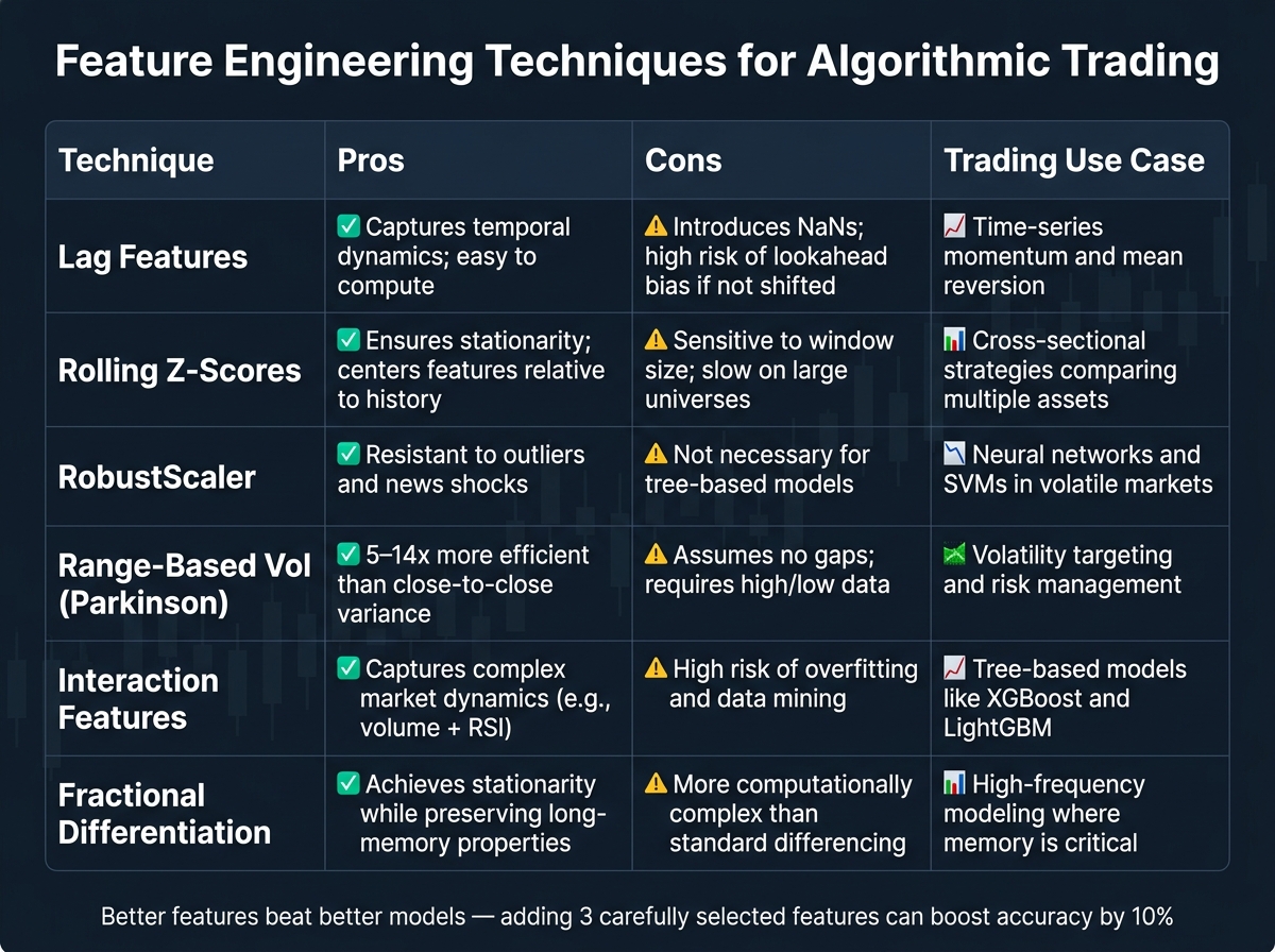
Feature Engineering Techniques for Algorithmic Trading: Pros, Cons & Use Cases
This checklist brings together the key techniques we've discussed, organizing them into practical steps for feature validation before deployment. Start with a correlation sanity check to ensure your features are free of lookahead bias or computational errors. Refer back to earlier steps on data quality for guidance. Use temporal splitting during cross-validation - this ensures the training set always comes before the validation and test sets, avoiding any data leakage from random shuffling.
One critical benchmark to keep in mind: because financial research has already explored a massive number of factors, a t-statistic above 3.0 is now the accepted threshold for true significance, rather than the traditional 2.0. As Campbell R. Harvey and colleagues explain:
"A t-statistic > 3.0 is required to establish true significance [to account for the factor zoo]."
Here’s a table summarizing the techniques covered, along with their strengths, weaknesses, and ideal trading applications:
| Technique | Pros | Cons | Trading Use Case |
|---|---|---|---|
| Lag Features | Captures temporal dynamics; easy to compute | Introduces NaNs; high risk of lookahead bias if not shifted | Time-series momentum and mean reversion |
| Rolling Z-Scores | Ensures stationarity; centers features relative to history | Sensitive to window size; slow on large universes | Cross-sectional strategies comparing multiple assets |
| RobustScaler | Resistant to outliers and news shocks | Not necessary for tree-based models | Neural networks and SVMs in volatile markets |
| Range-Based Vol (Parkinson) | 5–14x more efficient than close-to-close variance | Assumes no gaps; requires high/low data | Volatility targeting and risk management |
| Interaction Features | Captures complex market dynamics (e.g., volume + RSI) | High risk of overfitting and data mining | Tree-based models like XGBoost and LightGBM |
| Fractional Differentiation | Achieves stationarity while preserving long-memory properties | More computationally complex than standard differencing | High-frequency modeling where memory is critical |
This table can serve as a final checklist for validating your features.
Tip: Begin with 30–50 candidate features and narrow them down to the top 10–20 using methods like Permutation Importance or Mutual Information. Adding just three carefully selected features can boost model accuracy by 10%, while switching to a more complex algorithm might only yield a 1–3% improvement. As emphasized earlier, rigorous validation - using temporal splits, VIF analysis, and precise IC measurement - is critical for success in live trading. Ultimately, the quality of your features will always outweigh the complexity of your model.
FAQs
How do I know if a feature is leaking future data?
Feature leakage happens when a feature includes information that wouldn't be available at the time of prediction - like future returns or post-event statistics. This can skew testing results, making performance seem better than it actually is, and lead to poor outcomes in live trading.
To prevent this, always build features using only the data available up to the point of prediction. This ensures your model remains realistic and performs reliably in real-world scenarios.
What lookback window should I use for my indicators?
For short-term predictions, it's best to use a lookback window ranging from 1 to 48 periods. Extending beyond this range can lead to a higher chance of errors stacking up. Keeping the window shorter follows established best practices in feature engineering for trading.
How many features should I start with, and how do I cut them down?
When starting with features, there's no magic number, but aiming for a smaller, focused set - around 10 to 20 - is a good place to begin. This approach makes it easier to manage and refine your model. To identify and eliminate redundant or less useful features, you can rely on techniques like feature importance metrics, correlation analysis, or model-based methods. By iterating through this process, you can sharpen your model's performance, ensuring the feature set remains efficient and geared toward delivering strong predictive results.