Handling Missing Data in Price Series: 5 Methods

Handling Missing Data in Price Series: 5 Methods
If your trading results seem unreliable, missing data could be the problem. Gaps in historical price series - often displayed as NaN values - can disrupt calculations, distort backtests, and lead to inaccurate trading signals. These gaps arise from reasons like market holidays, trading halts, or data feed issues. Here’s a breakdown of five methods to address missing data effectively:
- Deletion: Remove rows with missing data. Best for small gaps in large datasets. Be cautious of disrupting time continuity.
- Mean, Median, or Constant Value Imputation: Fill gaps with averages or fixed values. Avoid look-ahead bias by using rolling windows.
- Forward Fill (LOCF): Carry the last known value forward. Works well for price data but may introduce artificial price jumps.
- Interpolation: Estimate values between known points. Suitable for small gaps but not for live trading due to reliance on future data.
- Model-Based/Multi-Asset Imputation: Use advanced techniques like KNN or correlations between assets to predict missing values. Ideal for longer gaps but computationally intensive.
Each method has its strengths and limitations. Choose based on the type of data, gap size, and whether you're backtesting or working in live markets. Proper handling of missing data ensures reliable results and better trading performance.
Missing Data Imputation: Mean, Median & KNN Explained
sbb-itb-3b27815
Missing Data Patterns in Price Series
Missing data in price series can show up in different ways. Sometimes, it's an entirely absent bar of data. Other times, it's a specific field missing - like a null Volume value while the OHLC (Open, High, Low, Close) data remains intact. Each scenario calls for its own solution.
It's crucial to distinguish between structural gaps and true data loss. Structural gaps are predictable and expected - think weekends, market holidays, or overnight closures. These gaps are normal and should remain in your dataset. On the other hand, true data loss comes from unexpected issues, like feed interruptions, transmission errors, or even vendor corrections. Even top-tier providers like Bloomberg or Refinitiv aren't immune to inconsistencies in historical data, especially when retroactive corrections have been applied unevenly. Misinterpreting a market holiday closure as a data error - or vice versa - can lead to flawed analyses.
Understanding the mechanisms behind missing data can help you decide how to handle it. These mechanisms fall into three categories:
| Mechanism | Cause | Example |
|---|---|---|
| MCAR (Missing Completely at Random) | No systematic reason; unrelated to any specific value | Random corruption during data transmission |
| MAR (Missing at Random) | Linked to other observed variables but not the missing value itself | A feed goes offline for scheduled maintenance |
| MNAR (Missing Not at Random) | The missing data depends on its own value | A stock halted during a volatile price spike |
MNAR poses the biggest challenge. For instance, if a stock’s price data vanishes during a spike, imputing that gap could hide critical volatility. This can skew your risk metrics in ways that are hard to detect.
"Data that is missing because a market was closed... requires a fundamentally different treatment than data missing because a stock was halted during extreme volatility." - asmr.education
Before jumping into fixes, it’s smart to run diagnostics. In Python, you can use df.isna().sum() to count gaps in each column. Plotting these gaps against a datetime index helps identify whether they cluster on specific dates (likely structural gaps) or appear scattered (likely true data loss). For intraday data, resampling to daily frequency and counting non-null values can highlight days with unusually thin coverage. Here's a tip: if Volume is missing, it often means zero trading activity. Replace it with 0 instead of forward-filling it like you would with a price. Forward-filling volume introduces false liquidity into your backtests, which can distort results.
Spotting these patterns is the first step to choosing the right cleaning method, which we'll dive into next.
1. Deleting Affected Bars or Segments
One of the quickest ways to address missing data is simply removing the affected rows. This approach works best when your dataset is large and the missing values are minimal. For example, if you’re dealing with years of tick data and only a few bars are corrupted, dropping them won’t significantly impact your analysis. As Haden Pelletier explains:
"If you have a lot of data, and not that many nulls, dropping a few rows won't make a huge difference. In this case, dropping is usually my preferred method since all the data I'll be feeding into the model is actual data."
This method is particularly useful when data accuracy is crucial - like in training machine learning models or handling Missing Not At Random (MNAR) gaps, such as trading halts during extreme market volatility. In these cases, imputing data could obscure critical risks.
However, deletion isn’t without drawbacks. One major issue is disrupted temporal continuity. Models like ARIMA or LSTM rely on evenly spaced time intervals. Removing just 10 bars from a 252-day return series could throw off your volatility and autocorrelation calculations, making them unrepresentative of a full trading year. Also, avoid calculating price differences before dropping rows with NaN values; this can distort cumulative price moves. For instance, a simulated random walk’s mean might shift from $0.20 to $0.14, skewing your results.
To minimize unnecessary data loss, use the subset parameter in dropna() to target specific columns - like the primary price feed or key strategy signals. For multi-asset datasets, avoid dropping rows with any NaN values, as this could lead to losing valuable information from unaffected data points.
2. Mean, Median, and Constant Value Imputation
When deletion methods aren't practical, statistical imputation techniques like mean, median, or constant value replacement can help fill data gaps while balancing continuity and accuracy. These approaches include mean imputation (replacing gaps with the average of available data), median imputation (using the middle value to avoid the influence of outliers), and constant value imputation (filling gaps with a fixed value, such as zero).
However, there's a major pitfall to watch out for: look-ahead bias. If you calculate a global mean or median from the entire dataset and use it to fill earlier gaps, you're effectively inserting future information into past data. Vladimir Kirilin, Quant Researcher at Five Rings Capital, explains:
"If you just use all-sample mean, you introduce an obvious look-ahead bias - i.e. you use future data to impute past values."
This kind of bias can artificially inflate backtest results by incorporating future data that wouldn't have been available at the time. To avoid this, use rolling or expanding windows. These methods - accessible via Pandas' rolling() or expanding() functions - calculate means and medians based only on data available up to the point of the gap, ensuring your backtest remains unbiased.
Beyond bias, imputation can also disrupt the natural flow of financial data. For example, mean and median imputation can create artificial price jumps if the imputed value deviates significantly from the last known price. This can trigger misleading signals in strategies that rely on momentum or mean reversion. Since financial prices often behave as martingales - where the best estimate for the next price is the current one - mean imputation's assumption of reversion to a long-term average doesn't align with how prices typically move.
Constant value imputation presents a different scenario depending on the type of data. For price data, it's rarely suitable. However, for volume data, filling gaps with zero is often the correct approach. A missing value in a volume series usually indicates no trading activity, so forward-filling or interpolating would inaccurately suggest trades that never happened.
Here's a quick breakdown of the strengths and limitations of each method:
| Method | Best Use Case | Key Limitation |
|---|---|---|
| Mean Imputation | Stationary series or local rolling windows | Introduces look-ahead bias; ignores temporal trends |
| Median Imputation | Series with significant outliers | Can create artificial steps or price jumps |
| Constant (Zero) | Volume data or indicator flags | Destructive if used for price data |
| Constant (Fixed Price) | Structural breaks or delisting scenarios | Fails to capture market volatility or drift |
For price data, always apply mean or median imputation after splitting training and test sets, and rely on rolling windows rather than global statistics. For volume data, fill gaps with zero - never with a mean or forward-fill. Choosing the right imputation method is critical for ensuring the integrity of your data and the reliability of your backtests.
Next, we'll look at methods that use adjacent values to maintain smoother continuity in your datasets.
3. Forward Fill and Backward Fill
Forward fill (or Last Observation Carried Forward, LOCF) is a method where the most recent known value is carried forward until a new value is observed. In Python's pandas library, you can implement this using df.ffill(). On the other hand, backward fill (df.bfill()) fills missing data using the next available value.
For financial data, forward fill aligns well with market theory. This approach is consistent with the martingale theory, which describes stock price movements. Vladimir Kirilin, a Quant Researcher at Five Rings Capital, elaborates:
"A more fundamental view on why LOCF is particularly suitable for stock price data is that it's usually modeled as a martingale. Roughly speaking, a martingale is something where our best guess for tomorrow is what we see today."
In simpler terms, if no new trade has occurred, the last traded price is often the best estimate for the current price. Forward fill reflects this assumption perfectly.
On the flip side, backward fill introduces potential pitfalls. By using future data to fill past gaps, it creates a look-ahead bias. This bias can inflate backtest results, making strategies appear more effective than they would be in real-world trading. For this reason, forward fill is the preferred method for both trading and backtesting, while backward fill is generally avoided in these scenarios.
That said, forward fill isn't without its challenges. One major issue is the artificial price jump that can occur when a gap ends. For instance, if a stock is forward-filled at $150.00 for several bars and then resumes trading at $132.00, the strategy might record a sudden drop that never actually happened in a single trading session. This can distort backtests and produce misleading trading signals. Another concern is the zero-volatility problem: forward-filling during market closures creates a flat line in the data, which can skew correlation and risk calculations. To mitigate these risks, you can use pandas' limit argument (e.g., df.ffill(limit=5)), which restricts the number of consecutive bars filled, reducing the propagation of outdated prices.
4. Interpolation Methods for Price Data
Interpolation offers a way to estimate price movements between observed points, creating a more natural price path during gaps instead of assuming prices remained static. Pandas' interpolate() method defaults to linear interpolation, making it a straightforward option to implement right away.
Different interpolation techniques work best in specific scenarios. Linear interpolation connects two known prices with a straight line, providing quick results but assuming a constant rate of price change - a pattern rarely seen in real markets. Spline interpolation uses smooth curves, making it ideal for yield curves or implied volatility surfaces. Meanwhile, polynomial interpolation can capture more intricate trends but risks overfitting or producing unrealistic outcomes like negative prices.
| Method | Best Use Case | Limitation |
|---|---|---|
| Linear | Short intraday gaps, small price changes | Struggles with non-linear volatility |
| Spline | Yield curves, implied volatilities | Higher computational demands |
| Polynomial | Complex, curved market trends | Prone to overfitting; may generate invalid values |
| Time-Weighted | Irregularly spaced trade data | Requires precise datetime indexing |
One key drawback of interpolation in backtesting is look-ahead bias. Unlike forward fill, interpolation relies on future data points to reconstruct past prices, making it unsuitable for live or real-time scenarios. Vladimir Kirilin, Quant Researcher at Five Rings Capital, highlights this limitation:
"Especially for a 'live' usage, interpolation is not really possible! After all, if today is day #93, how can we interpolate using a future value recorded at the end of day #95?"
Another issue is that interpolation often smooths out genuine volatility. Sudden price jumps or news-driven spikes during gaps may be erased, leading risk models to underestimate metrics like Value at Risk (VaR) and Expected Shortfall. To mitigate this, you can use Pandas' limit parameter to restrict the number of consecutive NaNs filled. Typically, filling beyond 6–10 bars introduces too much uncertainty to be reliable. It's also important to note that interpolation should be limited to price data and not applied to volume data.
Next, we’ll dive into model-based and multi-asset imputation methods that provide even more advanced approaches to data restoration.
5. Model-Based and Multi-Asset Imputation
When simpler approaches don't quite cut it - especially for longer data gaps or assets that tend to move together - model-based and multi-asset imputation steps in as a more refined option. These methods use correlations between assets and additional features to predict missing values, offering a more nuanced solution.
Two popular techniques stand out here: K-Nearest Neighbors (KNN) and Iterative Imputation. KNN works by identifying similar observations to fill in the blanks, while Iterative Imputation models each missing feature using all the others. This process involves repeated regression until the results stabilize. As Marco Cerliani explains:
"Using a knn or an iterative imputation, we can replicate the seasonality patterns and the underlying dynamics present in the data."
– Marco Cerliani
Taking it a step further, multi-asset imputation looks at the bigger picture by leveraging correlations between different instruments. For instance, if there's a gap in the 5-year Treasury yield, it can be estimated using data from the 2-year and 10-year yields through multivariate regression. Similarly, in equities, stocks that share common risk factors can help inform each other's missing values. The overarching idea here is:
"The key principle is that the imputation method should respect the economic relationships in the data, not just the statistical ones."
– asmr.education
However, these advanced methods come with their own set of challenges. They are more complex and require careful implementation, such as using tools like Scikit-learn's IterativeImputer. One critical concern is avoiding look-ahead bias. Models must only use data available up to the point of the gap:
"Any imputation that relies on global statistics (mean, median, regression coefficients) must be fit only on data available up to the point of the gap."
– asmr.education
Another potential drawback is the risk of creating feedback loops, which can artificially boost backtest performance and mask actual volatility spikes. These methods might inadvertently smooth over genuine market turbulence, underestimating tail risk. As a result, they are best suited for filling in multi-day gaps in assets that show strong, measurable correlations with others.
How to Pick the Right Method for Your Strategy
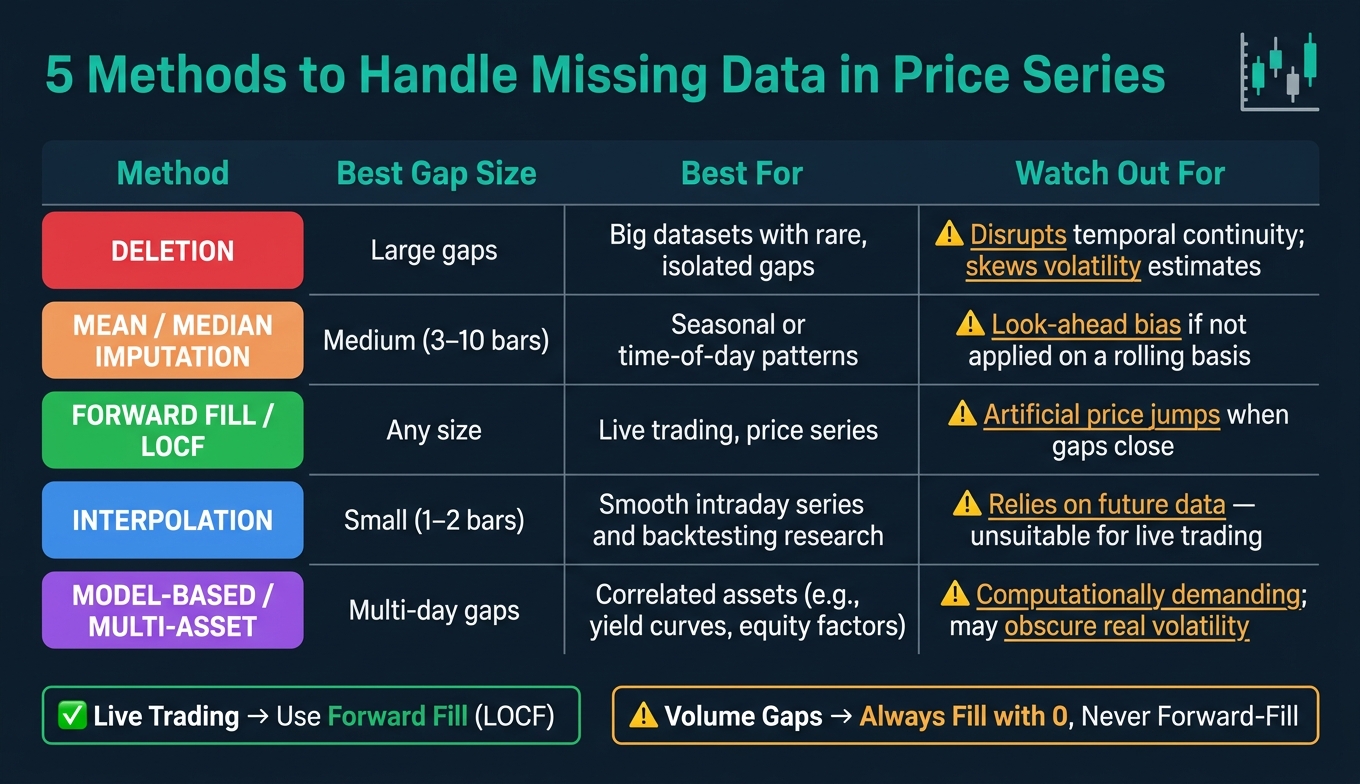
5 Methods to Handle Missing Data in Price Series: Quick Comparison Guide
When choosing a method for handling data gaps, it's important to recognize that no single approach works for every situation. The best method depends on factors like the length of the gap, the type of asset being analyzed, and whether you're backtesting or running live strategies.
Data scientist Haden Pelletier offers this insight:
"For small gaps (1–2 missing rows) that show up sporadically across the dataset, I will typically use interpolation. If the gaps are larger, though, with lots of consecutive nulls I would consider using the median up until a certain threshold."
To put this into practice: use interpolation for small, sporadic gaps (1–2 rows), and opt for median imputation for longer, consecutive gaps - up to a reasonable threshold. The table below provides a quick guide to match each method with its ideal use case:
| Method | Best Gap Size | Best For | Watch Out For |
|---|---|---|---|
| Deletion | Large gaps | Big datasets with rare gaps | Can disrupt continuity and skew volatility estimates |
| Mean/Median Imputation | Medium (3–10 bars) | Seasonal or time-of-day patterns | Risk of look-ahead bias if not applied on a rolling basis |
| Forward Fill (LOCF) | Any | Live trading, price series | May create artificial price jumps when gaps close |
| Interpolation | Small (1–2 bars) | Smooth intraday series and backtesting research | Relies on future data, making it unsuitable for live trading |
| Model-Based / Multi-Asset | Multi-day | Correlated assets (e.g., yield curves, equity factors) | Computationally demanding and may obscure real volatility |
This breakdown helps you pick the right approach for any given situation. A key takeaway: Forward fill is the go-to method for live trading, while interpolation is reserved for offline research. Using future data for gap filling in live strategies is a clear example of data leakage and should always be avoided.
For volume data, gaps should always be filled with 0, as missing volume typically indicates no activity rather than an unknown value. This ensures indicators like VWAP remain accurate and undistorted.
When transitioning from research to live execution, consistent preprocessing is essential. For example, in MQL5 workflows, a NaN value propagating through a moving average can silently erase an entire indicator output. If you're using tools like Traidies to generate MQL5 code and run automated backtests, ensure the same imputation logic is applied during both data preparation and strategy execution. This prevents discrepancies between clean backtest data and the tick-by-tick realities of live trading.
Conclusion
Missing data in price series can throw off calculations, distort backtests, and trigger misleading signals. Even a single missing data point among 10,000 rows can disrupt an analytical pipeline, leading to inaccurate returns, volatility estimates, Sharpe ratios, or correlation matrices.
The five methods discussed in this article each have their own strengths and are suited to specific scenarios. While no single approach works for every situation, the key takeaway is this: your chosen method must align with the size of the gap, the type of data, and whether you're working in an offline or live environment. This decision is critical - it’s what makes the difference between a backtest you can trust and one that’s only impressive on paper. Ensuring the right approach to handling missing data is fundamental for maintaining data integrity and achieving reliable trading performance.
Accurate historical data becomes even more crucial when running automated backtests. For instance, if you're using Traidies to generate MQL5 code and test strategies against historical price data, the quality of that data directly impacts the reliability of your results. Overlooking gaps or handling them poorly can lead to skewed performance metrics. A strategy that seems profitable in testing may behave unpredictably in live markets if the gaps weren’t addressed properly.
"The care taken with missing data often separates robust systems from fragile ones." - ASMR Education
Make data preprocessing a priority in your strategy development process. By carefully matching your imputation method to the specific needs of your strategy, you build a stronger foundation that protects against the risks of incomplete data. Investing time upfront to handle gaps correctly leads to more reliable signals, more trustworthy backtests, and strategies that hold up when it matters most - in live trading.
FAQs
How can I tell a market holiday gap from bad data?
Market holiday gaps happen during scheduled holidays when trading halts, leading to noticeable price changes without any activity during the break. To identify these, compare the gap with holiday calendars or official market closure schedules.
In contrast, bad data gaps appear randomly and lack an obvious explanation. These often include irregularities like inconsistent pricing. Verifying against official schedules can help distinguish between a holiday gap and a data error.
Which missing-data method is safest for live trading?
The safest way to handle missing data during live trading is using forward fill, also known as Last Observation Carried Forward (LOCF). This method keeps data consistent by filling in gaps with the most recent known value, preventing abrupt jumps in your dataset. However, it’s worth noting that this approach might not work well for highly volatile data, as it doesn’t reflect sudden market shifts. Ultimately, the best method depends on the specific characteristics of your data and your trading strategy.
How can I fill gaps without look-ahead bias?
To steer clear of look-ahead bias when filling gaps in time series, stick to techniques that rely solely on past data. One popular method is forward fill, where the most recent known value is carried forward. For smaller gaps, linear interpolation can be effective, as long as it doesn't pull in future data. It's best to avoid dropping data or using models that depend on future information unless they're explicitly designed to eliminate bias.